


Last week I presented a simple model that I used to predict the change, in basis points, in the SNB’s policy rate at its meeting later this week. I concluded that while the model suggested that the SNB will cut interest rates by 25 bps, there was a substantial probability that it will cut them by 50 bps.
In July I presented another model of SNB interest rate setting. In this post I look at what that model suggests the SNB will decide about interest rates this week. But first I will discuss how these models are best used to analyse upcoming monetary policy decisions.
Economic models
The best way to think of an economic model is as a map. Maps always involve simplifications – maps drawn on a scale of one-to-one are useless. Some information is amplified, and other information is disregarded. And maps are used for different purposes: a hiking map for Switzerland will contain very different information from an air traffic control map like the one above, but both will be useful for their intended purposes. This is true also for the various back-of-the-envelope econometric models of central bank policy decisions that I discuss here.
In my view, these models are best thought of as a nail in the wall that can be used to hang a painting on – not as the painting itself. Models are intended to add an element to a discussion, and not to short-cut that discussion. And one must never lose sight of the fact that models are always literally wrong since they involve simplifications.
Nevertheless, while point forecasts of models should be taken with a grain of salt, models can be useful for highlighting important questions to ask. Does the model’s prediction match up with what other commentators think? Why not? Does the model focus on the factors that seem to be most important now? Is it disregarding some essential elements in the current situation? What are those? How might they impact on a forecast?
With these caveats in mind, let’s return to the model.
Last week’s model
Last week’s model of SNB interest setting started from the observation that different central banks often change policy in the same direction and at about the same time. The reason for this is that their economies are often – but not always – affected by global economic developments and common external shocks. If you want to capture changes in the external economic environment the small and highly open Swiss economy faces, then using changes in the ECB’s and Federal Reserve’s policy rates is a good way to do that. But, of course, that doesn’t mean that the SNB passively follows what the ECB and the Federal Reserve decide.
Historically, the SNB has been keen avoid episodes of strong upward pressure on the franc, since they could lead to deflation and recession in Switzerland. Last week’s model therefore included a measure of the strength of the Swiss franc against the euro.
I estimated that model on quarterly data starting in 2000. I used quarterly data because the SNB sets interest rates quarterly and because interest rate cuts often happen in the same quarter, but not always in the same month. And I started in 2000 because episodes in which cuts coincide are important but do not happen every year.
Overall, last week’s model focussed on the external environment and the exchange rate of the franc. That seems appropriate in the current situation in which many observers worry about the likelihood of a global slowdown and the pressure on the franc to appreciate.
That model predicted a 32 bps cut in the SNB’s policy rate this quarter (given the 50 bps cut by the Fed and the 25 bps cut of the ECB).
My earlier model
My earlier model was quite different. The July model’s sole driving variable was the Swiss inflation rate. It also allowed for complicated dynamics in that the change in policy rate at one meeting affected the change in the policy rate at the next meeting. Moreover, the lagged interest rate mattered. (To be more precise, the difference between that lagged interest rate and the lagged inflation rate – the lagged real interest rate – mattered.)
That model was estimated on monthly data for the months in which the SNB had a policy meeting, starting in March 2021. It was intended to capture how the SNB has managed policy in the recent past when the key concern has been to offset the surge in inflation.
In this post I will update that model and explore what it predicts the SNB will announce on Thursday morning. Since this model disregards external factors and exchange market pressures that are at play currently, one would expect it to predict a smaller interest rate change than last week’s model.
Updating the July model
Updating the model entails reestimating it, adding the data point for June.1 I will also consider a few different measures of inflation:
Headline CPI inflation, which I used in the first version.
Domestic inflation.
Imported inflation. This measure of inflation is heavily impacted by exchange rate and thus incorporates that important channel.
Core inflation. The SNB never refers to core inflation in explaining policy, so I doubt that it plays an important role.
Inflation ex rents. Many commentators have noted that inflation is much lower if rents are disregarded.
The figure below shows these measures of inflation. They behave in broadly similar ways but indicate quite different price pressures in August. From low to high, the inflation rates are as follows: imported inflation -1.9%, inflation ex rent 0.4%, total and core inflation 1.1% and domestic inflation 2.0%.

Source BfS
Interestingly, when reestimating the model it became apparent that it fits best if inflation is measured excluding rents. That finding should not be overemphasised. My interpretation is that since the SNB recognises that interest rate increases mechanically raise CPI inflation, its assessment of price pressures may simply be better captured by CPI inflation ex rents than total CPI inflation during this specific period of large interest rate changes. To be clear, I am not saying that the SNB targets inflation ex rents.
Predictions
Next, I use this model to compute a forecast for how the SNB will change the interest rate this week. I start by computing a prediction when total CPI inflation is used and then turn to CPI inflation ex rents.
It is useful to start by reviewing the point estimates and associated standard errors of the three models. While last week’s model predicted a cut of 32 bps, the July model predicts a cut of 26 bps if inflation is used, and 30 bps if inflation ex rent is used. That implies that the July model will view a 50 bps cut as less likely than last week’s model.
Furthermore, the standard errors associated with both versions of the July model are smaller, 0.15, than that for last week’s model, 0.23. That implies that it will attach a lower probability to more extreme policy decisions. Since the probability of a 50 bps cut depends on the probability of an outcome between -37.5 bps and -62.5 bps, the model will attach a lower probability to a 50 bps cut.

Source: my estimates as described in the text.
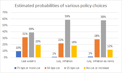
The graph below shows the probabilities. These are estimates and they could well be wrong. But they may nevertheless contain some information about what the SNB might decide later this week.
Source: my estimates as described in the text.
The histogram on the left shows again the results for the model I presented last week. Recall that it focussed on the SNB changing interest rates at the same time as the ECB and the Fed, and on the exchange rate. Since the standard error for the forecast is quite large, the model attaches a relatively high probability to extreme outcomes in the form of a 75 bps cut or interest rates being left unchanged or even increased. The main result is that while a 50 bps cut is less likely than a 25 bps cut, the difference is not that large (and certainly smaller than I anticipated).
The histogram in the middle shows the result for the model I presented in July, in the case in which total inflation is viewed as the single driver of SNB policy decisions. The key result is that that a 25 bps cut is about three times more likely than a 50 bps cut. Moreover, the extreme outcomes are seen as less likely than in the case of last week’s model.
Finally, the histogram on the right shows the result for the July model when inflation ex rents is used. In this case a 25 bps cut is about twice as likely as a 50 bps cut. The extreme outcomes are even less likely than in the earlier two cases.
Conclusions
What conclusions can we draw from this analysis? The main conclusion is that while a 25 bps cut seem most likely, there is a substantial probability of a 50 bps cut. Just how substantial is difficult to judge.
But these models disregard important factors. For instance, last week’s model incorporates the change in the Swiss franc against the euro over the last quarter. It thus neglects the fact that the exchange rate is at approximately the same level as a year ago. How important is that?
All models ignore the recent softening of the Swiss labour market. How concerned, if at all, will the SNB be about that? Similarly, the models disregard the likelihood that the Federal Reserve and perhaps also the ECB may cut interest rates before the next SNB meeting in December. Will the SNB be worried about that?
All in all, models may be helpful for analysing monetary policy decisions, but they still leave ample room for judgement.
The views expressed are my own. The work reported is preliminary and may be subject to errors. It should not be seen as constituting investment advice. Readers are advised to seek professional investment advice.
In the earlier draft I used inflation lagged two months as the driver of SNB decisions since that was marginally more significant than inflation lagged one month; here I use inflation lagged one month. Furthermore, in the earlier draft I constrained r* to equal -1%; here I estimate it freely.